Searching and Sorting

|

|
Searching
Hashing
Sorting
6.2 Searching
We will now turn our attention to some of the most common problems that arise in computing, those of searching and sorting.
Searching is the algorithmic process of finding a particular item in a collection of items. A search typically returns either True or False when queried on whether an item is present.
In Python, there is a very easy way to ask whether an item is in a list of items. We use the in operator.
using namespace std;
vector<int> v = {3, 5, 2, 4, 1};
cout << boolalpha << (find(v.begin(), v.end(), 15) != v.end()) << endl;
false
using namespace std;
vector<int> v = {3, 5, 2, 4, 1};
cout << boolalpha << (find(v.begin(), v.end(), 3) != v.end()) << endl;
true
Even though this is easy to write, an underlying process must be carried out to answer the question. It turns out that there are many different ways to search for the item!
6.3 The Sequential Search
When data items are stored in a collection such as a vector, we say that they have a linear or sequential relationship. The relative positions can be access using the index values of the individual items.
Since these index values are ordered, it is possible for us to visit them in sequence. This process gives rise to our first search technique, the sequential search.
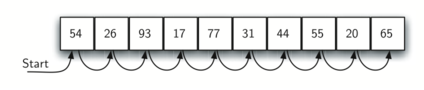
The following function needs two items – the list and the item we are looking for – and returns a Boolean value as to whether it is present.
#include <iostream>
#include <vector>
using namespace std;

bool sequentialSearch(vector<int> aList, int item) {
    unsigned pos = 0;
    while (pos < aList.size()) {
        if (aList[pos] == item) {
            return true;
        }
        pos = pos + 1;
    }
    return false;
}

int main() {
    vector<int> testList = {54, 26, 93, 17, 77, 31, 44, 55, 20, 65};
    cout << boolalpha;
    cout << sequentialSearch(testList, 44) << endl;
    cout << sequentialSearch(testList, 50) << endl;
    return 0;
}
true
false
6.3.1 Analysis of Sequential Search
To analyze searching algorithms, we need to decide on a basic unit of computation. For searching, it makes sense to count the number of comparisons performed.
Another assumption is that the probability that the item we are looking for is in any particular position is exactly the same for each position of the list.
If the item is not in the list, the only way to know that is to compare it against every item present. If there are $n$ items, then the sequential search requires $n$ comparisons to discover that the item is not there.
There are different scenarios that can occur if the item is in the list. In the best case we will find the item in the first place we look, at the beginning of the list. We will need only one comparison. In the worst case, we will not discover the item until the very last comparison, the $n$-th comparison.
On average, we will find the item about half way into the list; that is, we will compare against $\frac{n}{2}$ items. So the complexity of the sequential search is $O(n)$
What would happen to the sequential search if the items were ordered in some way? Would we be able to gain any efficiency in our search technique?
Assume that the list of items was constructed so that the items are in ascending order, from low to high. If the item we are looking for is present in the list, the chance of it is still the same as before.
If the item is not present there is a slight advantage!
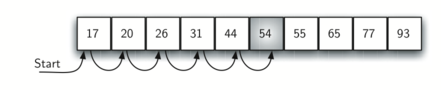
If we are search for 50 no other elements beyond 54 can work. In this case, the algorithm does not have to continue looking through all of the items to report that the item was not found. It can stop immediately!
#include <iostream>
#include <vector>
using namespace std;

bool orderedSequentialSearch(vector<int> aList, int item) {
    unsigned pos = 0;
    while (pos < aList.size()) {
        if (aList[pos] == item) return true;
        if (aList[pos] > item) return false;   // passed the spot: stop early!
        pos = pos + 1;
    }
    return false;
}

int main() {
    vector<int> testList = {17, 20, 26, 31, 44, 54, 55, 65, 77, 93};
    cout << boolalpha << orderedSequentialSearch(testList, 44) << endl;
    cout << orderedSequentialSearch(testList, 50) << endl;
    return 0;
}
true
false
The original complexity and the complexity of the ordered sequential search is as follows:
| Case | Best Case | Worst Case | Average Case |
|---|---|---|---|
| item is present | 1 | $n$ | $\frac{n}{2}$ |
| item is not present | $n$ | $n$ | $n$ |
| Case | Best Case | Worst Case | Average Case |
|---|---|---|---|
| item is present | 1 | $n$ | $\frac{n}{2}$ |
| item is not present | 1 | $n$ | $\frac{n}{2}$ |
However, this technique is still $O(n)$.
display_quiz(path+"sequential.json", max_width=800)
6.4 The Binary Search
It is possible to take greater advantage of the ordered list if we are clever with our comparisons. A binary search will start by examining the middle item. If that item is the one we are searching for, we are done.
If it is not the correct item, we can use the ordered nature of the list to eliminate half of the remaining items!
If the item we are searching for is greater than the middle item, we know that the entire first (left) half of the list as well as the middle item can be eliminated from further consideration. The item, if it is in the list, must be in the second (right) half.
We can then repeat the process with the left half. Start at the middle item and compare it against what we are looking for.
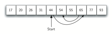
The figure above shows how this algorithm can quickly find the value 54.
bool binarySearch(vector<int> aList, int item) {
    int first = 0;
    int last = aList.size() - 1;
    while (first <= last) {
        int midpoint = (first + last) / 2;
        cout << midpoint - first << endl;   // how far the midpoint moved
        if (aList[midpoint] == item) return true;
        else if (item < aList[midpoint]) last = midpoint - 1;
        else first = midpoint + 1;
    }
    return false;
}
#include <iostream>
#include "dscpp/searching.hpp"   // the searches of this chapter
using namespace std;

int main() {
    vector<int> testList = {17, 20, 26, 31, 44, 54, 55, 65, 77, 93};
    cout << boolalpha;
    cout << binarySearch(testList, 44) << endl;
    cout << binarySearch(testList, 50) << endl;
    return 0;
}
4
true
4
2
0
false
This algorithm is a great example of a divide and conquer strategy. This means that we divide the problem into smaller pieces, solve the smaller pieces in some way, and then reassemble the whole problem to get the result.
This is a recursive call to the binary search function passing a smaller list.
bool binarySearchRec(vector<int> aList, int item) {
    if (aList.size() == 0) return false;
    int midpoint = (aList.size() - 1) / 2;   // different from the textbook!
    cout << aList[midpoint] << endl;
    if (aList[midpoint] == item) return true;
    if (item < aList[midpoint]) {
        vector<int> left(aList.begin(), aList.begin() + midpoint);
        return binarySearchRec(left, item);          // aList[:midpoint]
    }
    vector<int> right(aList.begin() + midpoint + 1, aList.end());
    return binarySearchRec(right, item);             // aList[midpoint+1:]
}
#include <iostream>
#include "dscpp/searching.hpp"
using namespace std;

int main() {
    vector<int> testList = {17, 20, 26, 31, 44, 54, 55, 65, 77, 93};
    cout << boolalpha;
    cout << binarySearchRec(testList, 44) << endl;
    cout << binarySearchRec(testList, 50) << endl;
    return 0;
}
44
true
44
65
54
false
6.4.1. Analysis of Binary Search
What is the maximum number of comparisons this algorithm will require to check the entire list? If we start with $n$ items, about $\frac{n}{2}$ items will be left after the first comparison. After the second comparison, there will be about $\frac{n}{4}$. Then $\frac{n}{8}$, and so on. How many times can we split the list?
| Comparisons | Approximate Number of Items Left |
|---|---|
| 1 | $\frac{n}{2}$ |
| 2 | $\frac{n}{4}$ |
| 3 | $\frac{n}{8}$ |
| ... | |
| $i$ | $\frac{n}{2^i}$ |
When we split the list enough times, we end up with a list that has just one item. Either that is the item we are looking for or it is not. The number of comparisons necessary to get to this point is $i$ where $\frac{n}{2^i}=1$.
Solving for $i$ gives us $i = \log n$. The maximum number of comparisons is logarithmic with respect to the number of items in the list. Therefore, the binary search is $O(\log n)$
Note that the recursive call binary_search_rec(a_list[:midpoint], item) uses slicing operator to create the left half of the list that is then passed to the next invocation. However, we know that in Python it is actually $O(k)$. This means that the binary search using slicing will not perform in strict logarithmic time. Luckily this can be remedied by passing the list along with the starting and ending indices. We leave this implementation as an exercise.
Even though a binary search is generally better than a sequential search, it is important to note that for small values of $n$, the additional cost of sorting is probably not worth it.
If we can sort once and then search many times, the cost of the sort is not so significant. However, for large lists, sorting even once can be so expensive that simply performing a sequential search from the start may be the best choice.
display_quiz(path+"binary.json", max_width=800)
Exercise 1: Implement the binary search using recursion without the slice operator. Recall that you will need to pass the list along with the starting and ending index values for the sublist.
#include <iostream>
#include <vector>
using namespace std;

bool binarySearchRec2(vector<int>& aList, int item, int start, int last) {
    if (____) return false;                 // base case: empty range
    int midpoint = ____;
    if (aList[midpoint] == item) return true;
    if (item < aList[midpoint]) return binarySearchRec2(____);
    return binarySearchRec2(____);
}
int main() {
    vector<int> t = {17, 20, 26, 31, 44, 54, 55, 65, 77, 93};
    cout << boolalpha << binarySearchRec2(t, 44, 0, t.size() - 1) << endl;
    return 0;
}
/tmp/tmpmm04vw9o.cpp: In function ‘bool binarySearchRec2(std::vector<int>&, int, int, int)’:
/tmp/tmpmm04vw9o.cpp:8:9: error: ‘____’ was not declared in this scope
    8 |     if (____) return false;
      |         ^~~~
/tmp/tmpmm04vw9o.cpp:9:20: error: ‘____’ was not declared in this scope
    9 |     int midpoint = ____;
      |                    ^~~~
[C++ kernel] Error: Unable to compile the source code. Return error: 0x1.
Fix the recursive calls (and the midpoint computation) so the program compiles and finds 44 but not 50 — without creating any sub-vectors.
6.5 Hashing
In previous sections we were able to make improvements in our search algorithms by taking advantage of information about where items are stored in the collection with respect to one another. For example, by knowing that a list was ordered, we could search in logarithmic time using a binary search.
In this section we will attempt to go one step further by building a data structure that can be searched in $O(1)$ time. This concept is referred to as hashing.
A hash table is a collection of items which are stored in such a way as to make it easy to find them later. Each position of the hash table, often called a slot, can hold an item and is named by an integer value starting at 0.
For example, we will have a slot named 0, a slot named 1, a slot named 2, and so on. Initially, the hash table contains no items so every slot is empty. We can implement a hash table by using a list with each element initialized to None. Assume the size of the table is $m$.

The mapping between an item and the slot where that item belongs in the hash table is called the hash function. The hash function will take any item in the collection and return an integer in the range of slot names between 0 and $m-1$.
Assume that we have the set of integer items 54, 26, 93, 17, 77, and 31. Our first hash function, sometimes referred to as the remainder method, simply takes an item and divides it by the table size, returning the remainder as its hash value $h(item)=item \% 11$
| Item | Hash value |
|---|---|
| 54 | 10 |
| 26 | 4 |
| 93 | 5 |
| 17 | 6 |
| 77 | 0 |
| 31 | 9 |
Once the hash values have been computed, we can insert each item into the hash table at the designated position.
Note that 6 of the 11 slots are now occupied. This is referred to as the load factor, and is commonly denoted by $\lambda= \frac{number\ of\ items}{table\ size}=\frac{6}{11}$

Now when we want to search for an item, we simply use the hash function to compute the slot name for the item and then check the hash table to see if it is present. This searching operation is $O(1)$!
You can probably already see that this technique is going to work only if each item maps to a unique location in the hash table.
For example, if the item 44 had been the next item in our collection, it would have a hash value of 0 ($44 \% 11 = 0$). Since 77 also had a hash value of 0, we would have a problem!
According to the hash function, two or more items would need to be in the same slot. This is referred to as a collision (it may also be called a clash). Clearly, collisions create a problem for the hashing technique.
6.5.1. Hash Functions
Given a collection of items, a hash function that maps each item into a unique slot is referred to as a perfect hash function. Unfortunately, given an arbitrary collection of items, there is no systematic way to construct a perfect hash function. Luckily, we do not need the hash function to be perfect to still gain performance efficiency!
Our goal is to create a hash function that minimizes the number of collisions, is easy to compute, and evenly distributes the items in the hash table.
Note that this remainder method (modulo) will typically be present in some form in all hash functions since the result must be in the range of slot names.
The folding method for constructing hash functions begins by dividing the item into equal-sized pieces (the last piece may not be of equal size). These pieces are then added together to give the resulting hash value.
For example, if our item was the phone number 436-555-4601, we would take the digits and divide them into groups of 2 (43, 65, 55, 46, 01). After the addition, $43+65+55+46+01$, we get $210$. If we assume our hash table has 11 slots, then we need to perform the extra step of dividing by 11 and keeping the remainder.
In this case $210 \% 11$ is 1, so the phone number 436-555-4601 hashes to slot 1. Some folding methods go one step further and reverse every other piece before the addition. For the above example, we get $34+56+55+64+10=219$ which gives $219 \%11 =10$.
Another numerical technique for constructing a hash function is called the mid-square method. We first square the item, and then extract some portion of the resulting digits. For example, if the item were 44, we would first compute $44^2=1936$. By extracting the middle two digits, 93, and performing the remainder step, we get 5 $(93\%11)$.
| Item | Remainder | Mid-Square |
|---|---|---|
| 54 | 10 | 3 |
| 26 | 4 | 1 |
| 93 | 5 | 9 |
| 17 | 6 | 6 |
| 77 | 0 | 4 |
| 31 | 9 | 8 |
#include <iostream>
#include <string>
using namespace std;

int remainderMethod(int item, int divisor) { return item % divisor; }
int midsquareMethod(int item, int divisor) {
    string squared = to_string(item * item);
    if (squared.length() % 2 != 0) squared = "0" + squared;
    int mid = squared.length() / 2;
    return stoi(squared.substr(mid - 1, 2)) % divisor;
}

int main() {
    printf("%6s %10s %11s\n", "Item", "Remainder", "Mid-Square");
    for (int item : {54, 26, 93, 17})
        printf("%6d %10d %11d\n", item,
               remainderMethod(item, 11), midsquareMethod(item, 11));
    return 0;
}
Item Remainder Mid-Square
54         10           3

26          4           1

93          5           9

17          6           6
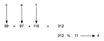
We can also create hash functions for character-based items such as strings. For example, the word "cat" can be thought of as a sequence of ordinal values. We can then take these three ordinal values, add them up, and use the remainder method to get a hash value.
#include <iostream>
#include <string>
using namespace std;

int hashStr(string aString, int tableSize) {
    int sum = 0;
    for (char c : aString) {
        sum = sum + int(c);   // the ordinal value of the character
    }
    return sum % tableSize;
}

int main() {
    cout << hashStr("cat", 11) << endl;
    return 0;
}
4
It is interesting to note that when using this hash function, anagrams will always be given the same hash value. To remedy this, we could use the position of the character as a weight.
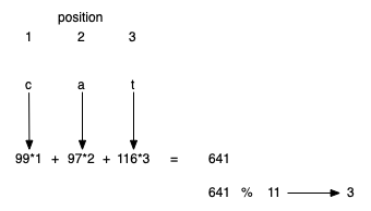
The important thing to remember is that the hash function has to be efficient so that it does not become the dominant part of the storage and search process. Otherwise, we could just use the search as before.
6.5.2. Collision Resolution
We now return to the problem of collisions. When two items hash to the same slot, we must have a systematic method for placing the second item in the hash table. This process is called collision resolution.
A simple way to do this is to start at the original hash value position and then move in a sequential manner through the slots until we encounter the first slot that is empty. Note that we may need to go back to the first slot (circularly) to cover the entire hash table.
This collision resolution process is referred to as open addressing in that it tries to find the next open slot or address in the hash table. By systematically visiting each slot one at a time, we are performing an open addressing technique called linear probing.
Consider an extended set of integer items under the simple remainder method hash function (54, 26, 93, 17, 77, 31, 44, 55, 20). The following is the placement of the original first six values:
Let's see what happens when we attempt to place the additional three items into the table. When we attempt to place 44 into slot 0, a collision occurs. Under linear probing, we look sequentially, slot by slot, until we find an open position. In this case, we find slot 1. We can also do the same thing for the other values:

Once we have built a hash table using open addressing and linear probing, it is essential that we utilize the same methods to search for items. If we are looking for 20 the hash value is 9, and slot 9 is currently holding 31. We cannot simply return False since we know that there could have been collisions. We are now forced to do a sequential search, starting at position 10, looking until either we find the item 20 or we find an empty slot!
A disadvantage to linear probing is the tendency for clustering; This means that if many collisions occur at the same hash value, a number of surrounding slots will be filled by the linear probing resolution.
This will have an impact on other items that are being inserted, as we saw when we tried to add the item 20 above. A cluster of values hashing to 0 had to be skipped to finally find an open position.

One way to deal with clustering is to extend the linear probing technique so that instead of looking sequentially for the next open slot, we skip slots, thereby more evenly distributing the items that have caused collisions. The following shows the items when collision resolution is done with what we will call a "plus 3" probe. This means that once a collision occurs, we will look at every third slot until we find one that is empty.

The general name for this process of looking for another slot after a collision is rehashing. With simple linear probing, the rehash function is $new\_hash=rehash(old\_hash), rehash(pos)=(pos+skip)\%size$.
It is important to note that the size of the skip must be such that all the slots in the table will eventually be visited. Otherwise, part of the table will be unused. To ensure this, it is often suggested that the table size be a prime number.
#include <iostream>
#include <vector>
using namespace std;

int main() {
    vector<int> items = {54, 26, 93, 17, 77, 31, 44, 55, 20};
    vector<int> hashTable(11, -1);            // -1 plays the role of None
    for (int item : items) {
        int hashIndex = item % 11;
        while (hashTable[hashIndex] != -1)    // linear probing on collision
            hashIndex = (hashIndex + 1) % 11;
        hashTable[hashIndex] = item;
    }
    for (int idx = 0; idx < 11; idx++)
        cout << idx << ":" << hashTable[idx] << "  ";   // slot:item
    cout << endl;
    return 0;
}
0:77 1:44 2:55 3:20 4:26 5:93 6:17 7:-1 8:-1 9:31 10:54
A variation of the linear probing idea is called quadratic probing. Instead of using a constant skip value, we use a rehash function that increments the hash value by 1, 4, 9 and so on.
This means that if the first hash value is $h$, the successive values are $h+1, h+4, h+9$, and so on. In other words, quadratic probing uses a skip consisting of successive perfect squares.

An alternative method for handling the collision problem is to allow each slot to hold a reference to a collection (or chain) of items. Chaining allows many items to exist at the same location in the hash table. When collisions happen, the item is still placed in the proper slot of the hash table. As more and more items hash to the same location, the difficulty of searching for the item in the collection increases.
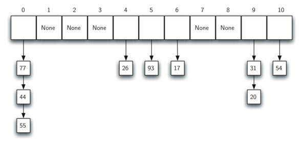
When we want to search for an item, we use the hash function to generate the slot where it should reside. Since with chaining each slot holds a collection, we use a searching technique to decide whether the item is present.
display_quiz(path+"hash1.json", max_width=800)
display_quiz(path+"hash2.json", max_width=800)
Exercise 2: Implement quadratic probing as a rehash technique
#include <iostream>
#include <vector>
using namespace std;

vector<int> quadraticProbing(vector<int> items, int divisor) {
    vector<int> hashTable(divisor, -1);   // -1 = empty
    for (int item : items) {
        int hashIndex = item % divisor;
        while (hashTable[hashIndex] != -1)
            hashIndex = ____;   // probe h, h+1, h+4, h+9, ...
        hashTable[hashIndex] = item;
    }
    return hashTable;
}
int main() {
    for (int v : quadraticProbing({113, 117, 97, 100, 114, 108, 116, 105, 99}, 11))
        cout << v << " ";
    return 0;
}
/tmp/tmp4id6bkj5.cpp: In function ‘std::vector<int> quadraticProbing(std::vector<int>, int)’:
/tmp/tmp4id6bkj5.cpp:12:25: error: ‘____’ was not declared in this scope
   12 |             hashIndex = ____;
      |                         ^~~~
[C++ kernel] Error: Unable to compile the source code. Return error: 0x1.
With quadratic probing the probe sequence is $h, h+1, h+4, h+9, \dots$ — complete the loop so the nine keys all land in distinct slots of the size-11 table.
6.5.3. Implementing the Map Abstract Data Type
One of the most useful C++ collections is the hash table (unordered_map). Recall that it is a data type that stores key-value pairs and lets you look up a value by its key in constant average time. We now build our own version, the map abstract data type.
The map abstract data type is defined as follows. The structure is an unordered collection of associations between a key and a data value.
Map()creates a new empty map.put(key, val)adds a new key–value pair to the map. If the key is already in the map, it replaces the old value with the new value.
get(key)takes a key and returns the matching value stored in the map or the empty string otherwise.deldeletes the key–value pair from the map using a statement of the formdel map[key].size()returns the number of key–value pairs stored in the map.inreturnTruefor a statement of the form key in map if the given key is in the map,Falseotherwise.
One of the great benefits of a dictionary is the fact that given a key, we can look up the associated data value very quickly. This could be done if we use a hash table as described above.
We use two lists to create a HashTable class that implements the map abstract data type. One list, called slots, will hold the key items and a parallel list, called data, will hold the data values. When we look up a key, the corresponding position in the data list will hold the associated data value.
class HashTable {
    public:
        HashTable(int sz) {
            size = sz;
            slots = vector<int>(size, -1);        // -1 marks an empty slot
            data = vector<string>(size, "");
        }

        int hashFunction(int key) {
            return key % size;
        }

        int rehash(int oldHash) {
            return (oldHash + 1) % size;
        }

    private:
        int size;
        vector<int> slots;
        vector<string> data;
};
void put(int key, string value) {
    int hashValue = hashFunction(key);

    if (slots[hashValue] == -1) {
        slots[hashValue] = key;
        data[hashValue] = value;
    } else {
        if (slots[hashValue] == key) {
            data[hashValue] = value;   // replace
        } else {
            int nextSlot = rehash(hashValue);
            while (slots[nextSlot] != -1 && slots[nextSlot] != key) {
                nextSlot = rehash(nextSlot);
            }
            slots[nextSlot] = key;
            data[nextSlot] = value;
        }
    }
}
hash_function() implements the simple remainder method. The collision resolution technique is linear probing with a "plus 1" rehash value. The put() function assumes that there will eventually be an empty slot. If a nonempty slot already contains the key, the old data value is replaced with the new data value.
string get(int key) {
    int startSlot = hashFunction(key);

    int position = startSlot;
    while (slots[position] != -1) {
        if (slots[position] == key) {
            return data[position];
        }
        position = rehash(position);
        if (position == startSlot) {
            return "";   // not found: return the empty string
        }
    }
    return "";
}
The get() function begins by computing the initial hash value. If the value is not in the initial slot, rehash is used to locate the next possible position. Notice that line 10 guarantees that the search will terminate by checking to make sure that we have not returned to the initial slot. If that happens, we have exhausted all possible slots and the item must not be present.
The following session shows the HashTable class in action.
The complete class is in pythonds3/cppds/searching/hash_table.cpp. Here it is in action:
#include <iostream>
#include "dscpp/hashtable.hpp"   // the class of this section
using namespace std;

int main() {
    HashTable h(11);
    int keys[] = {54, 26, 93, 17, 77, 31, 44, 55, 20};
    string vals[] = {"cat", "dog", "lion", "tiger", "bird",
                     "cow", "goat", "pig", "chicken"};
    for (int i = 0; i < 9; i++) h.put(keys[i], vals[i]);

    h.printSlots();
    h.printData();
    return 0;
}
77 44 55 20 26 93 17 -1 -1 31 54
bird goat pig chicken dog lion tiger - - cow cat
Next we will access and modify some items in the hash table. Note that the value for the key 20 is being replaced.
#include <iostream>
#include "dscpp/hashtable.hpp"
using namespace std;

int main() {
    HashTable h(11);
    int keys[] = {54, 26, 93, 17, 77, 31, 44, 55, 20};
    string vals[] = {"cat", "dog", "lion", "tiger", "bird",
                     "cow", "goat", "pig", "chicken"};
    for (int i = 0; i < 9; i++) h.put(keys[i], vals[i]);

    cout << h.get(20) << " " << h.get(17) << endl;
    h.put(20, "duck");                            // replace the value for key 20
    cout << h.get(20) << endl;
    h.printData();
    cout << "[" << h.get(99) << "]" << endl;      // not in the table: empty string
    return 0;
}
chicken tiger
duck
bird goat pig duck dog lion tiger - - cow cat
[]
6.5.4. Analysis of Hashing (Optional)
We stated earlier that in the best case hashing would provide an $O(1)$, constant time search technique. However, due to collisions, the number of comparisons is typically not so simple. A complete analysis of hashing is beyond the scope of this text, we state some well-known results that approximate the number of comparisons necessary to search for an item.
The most important piece of information we need to analyze the use of a hash table is the load factor $\lambda$. Conceptually, if $\lambda$ is small, then there is a lower chance of collisions, meaning that items are more likely to be in the slots where they belong.
If $\lambda$ is large, meaning that the table is filling up, then there are more and more collisions. This means that collision resolution is more difficult, requiring more comparisons to find an empty slot.
As before, we will have a result for both a successful and an unsuccessful search. For a successful search using open addressing with linear probing, the average number of comparisons is approximately $\frac{1}{2}\left(1+\frac{1}{1-\lambda}\right)$ and an unsuccessful search gives $\frac{1}{2}\left(1+\left(\frac{1}{1-\lambda}\right)^2\right)$.
If we are using chaining, the average number of comparisons is $1 + \frac {\lambda}{2}$ for the successful case, and simply $\lambda$ comparisons if the search is unsuccessful.
7.2 Sorting
Sorting is the process of placing elements from a collection in some kind of order. For example, a list of words could be sorted alphabetically or by length. We have already seen a number of algorithms that were able to benefit from having a sorted list (recall the anagram example and the binary search).
Sorting a large number of items can take a substantial amount of computing resources. Like searching, the efficiency of a sorting algorithm is related to the number of items being processed.
For small collections, a complex sorting method may be more trouble than it is worth. The overhead may be too high. On the other hand, for larger collections, we want to take advantage of as many improvements as possible.
In this section we will discuss several sorting techniques and compare them with respect to their running time.
We should think about the operations that can be used to analyze a sorting process. First, it will be necessary to compare two values to see which is smaller (or larger). In order to sort a collection, it will be necessary to have some systematic way to compare values to see if they are out of order. The total number of comparisons will be the most common way to measure a sort procedure.
Second, when values are not in the correct position with respect to one another, it may be necessary to exchange them. This exchange is a costly operation and the total number of exchanges will also be important for evaluating the overall efficiency of the algorithm.
7.3. The Bubble Sort
The bubble sort makes multiple passes through a list. It compares adjacent items and exchanges those that are out of order. Each pass through the list places the next largest value in its proper place. In essence, each item bubbles up to the location where it belongs.
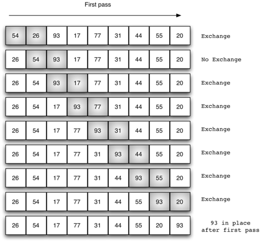
If there are $n$ items in the list, then there are $n-1$ pairs of items that need to be compared on the first pass.
At the start of the second pass, the largest value is now in place. There are $n-1$ items left to sort, meaning that there will be $n-2$ pairs. Since each pass places the next largest value in place, the total number of passes necessary will be $n-1$.
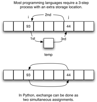
The exchange operation, sometimes called a swap, is slightly different in Python than in most other programming languages. Typically, swapping two elements in a list requires a temporary variable (an additional memory location).
temp = a_list[i]
a_list[i] = a_list[j]
a_list[j] = temp
Without the temporary storage, one of the values would be overwritten.
In C++, exchanging two values uses the swap() function from the standard library (or the classic three-step temporary-variable dance): swap(aList[j], aList[j + 1]);
#include <iostream>
#include "dscpp/sorting.hpp"   // printl + the sorts of this chapter
using namespace std;

int main() {
    vector<int> aList = {4, 14, 5, 21, 29, 12, 16};
    bubbleSort(aList);   // prints the vector at the start of every pass
    printl(aList);
    return 0;
}
4 14 5 21 29 12 16
4 5 14 21 12 16 29
4 5 14 12 16 21 29
4 5 12 14 16 21 29
4 5 12 14 16 21 29
4 5 12 14 16 21 29
4 5 12 14 16 21 29
To analyze the bubble sort, we should note that regardless of how the items are arranged in the initial list, $n-1$ passes will be made to sort a list of size $n$.
| Pass | Comparisons |
|---|---|
| 1 | n-1 |
| 2 | n-2 |
| 3 | n-3 |
... |
... |
| n-1 | 1 |
The total number of comparisons is the sum of the first $n$ integers which is $\frac{1}{2}n^{2} - \frac{1}{2}n$. This is $O(n^2)$ comparisons.
A bubble sort is often considered the most inefficient sorting method since it must exchange items before the final location is known. These "wasted" exchange operations are very costly.
However, because the bubble sort makes passes through the entire unsorted portion of the list, it has the capability to do something most sorting algorithms cannot. In particular, if during a pass there are no exchanges, then we know that the list must be sorted!
#include <iostream>
#include "dscpp/sorting.hpp"
using namespace std;

int main() {
    vector<int> aList = {20, 30, 40, 90, 50, 60, 70, 80, 100, 110};
    bubbleSortShort(aList);   // stops as soon as a pass makes no exchange
    printl(aList);
    return 0;
}
20 30 40 50 60 70 80 90 100 110
This is often called short bubble.
7.4. The Selection Sort
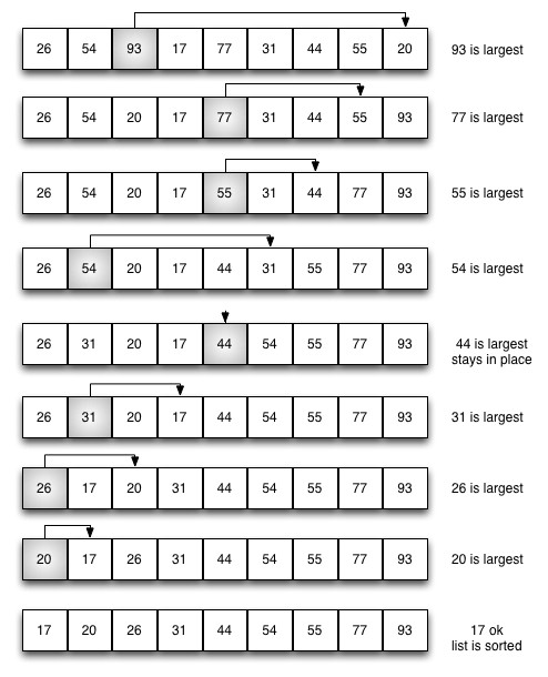
The selection sort improves on the bubble sort by making only one exchange for every pass through the list. Selection sort looks for the largest value as it makes a pass and, after completing the pass, places it in the proper location.
As with a bubble sort, after the first pass, the largest item is in the correct place. After the second pass, the next largest is in place. This process continues and requires $n-1$ passes to sort $n$ items, since the final item must be in place after the $n-1$ pass.
#include <iostream>
#include "dscpp/sorting.hpp"
using namespace std;

int main() {
    vector<int> aList = {11, 7, 12, 14, 19, 1, 6, 18, 8, 20};
    selectionSort(aList);   // prints the vector at the start of every pass
    printl(aList);
    return 0;
}
11 7 12 14 19 1 6 18 8 20
1 7 12 14 19 11 6 18 8 20
1 6 12 14 19 11 7 18 8 20
1 6 7 14 19 11 12 18 8 20
1 6 7 8 19 11 12 18 14 20
1 6 7 8 11 19 12 18 14 20
1 6 7 8 11 12 19 18 14 20
1 6 7 8 11 12 14 18 19 20
1 6 7 8 11 12 14 18 19 20
1 6 7 8 11 12 14 18 19 20
You may see that the selection sort makes the same number of comparisons as the bubble sort and is therefore also $O(n^2)$. However, due to the reduction in the number of exchanges, the selection sort typically executes faster in benchmark studies!
7.5 The Insertion Sort
The insertion sort, although still $O(n^2)$, works in a slightly different way. It always maintains a sorted sublist in the lower positions of the list. Each new item is then inserted back into the previous sublist such that the sorted sublist is one item larger.
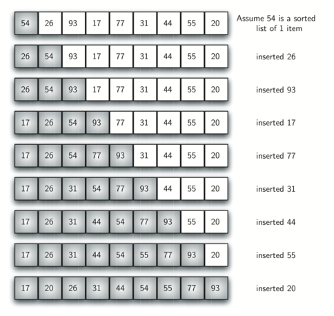
We begin by assuming that a list with one item (position $0$) is already sorted. On each pass, one for each item 1 through $n-1$, the current item is checked against those in the already sorted sublist.
As we look back into the already sorted sublist, we shift those items that are greater to the right. When we reach a smaller item or the end of the sublist, the current item can be inserted.
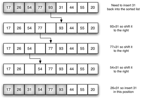
The implementation of insertion_sort() shows that there are again $n-1$ passes to sort $n$ items. The iteration starts at position 1 and moves through position $n-1$, as these are the items that need to be inserted back into the sorted sublists.
#include <iostream>
#include "dscpp/sorting.hpp"
using namespace std;

int main() {
    vector<int> aList = {9, 2, 5, 5, 7, 9, 1};
    insertionSort(aList);   // prints the vector before every insertion pass
    printl(aList);
    return 0;
}
9 2 5 5 7 9 1
2 9 5 5 7 9 1
2 5 9 5 7 9 1
2 5 5 9 7 9 1
2 5 5 7 9 9 1
2 5 5 7 9 9 1
1 2 5 5 7 9 9
One note about shifting versus exchanging is also important. In general, a shift operation requires approximately a third of the processing work of an exchange since only one assignment is performed. In benchmark studies, insertion sort will show very good performance.
7.6. The Shell Sort
The Shell sort, sometimes called the diminishing increment sort, improves on the insertion sort by breaking the original list into a number of smaller sublists, each of which is sorted using an insertion sort.
Instead of breaking the list into sublists of contiguous items, the Shell sort uses an increment $i$, sometimes called the gap, to create a sublist by choosing all items that are $i$ items apart. If we use an increment of three, there are three sublists, each of which can be sorted by an insertion sort.
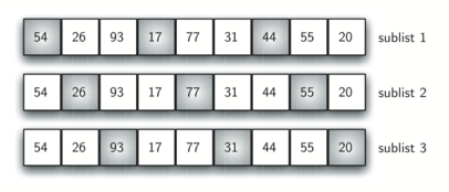
After completing these sorts, we get:
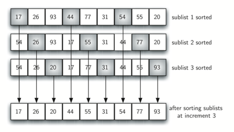
By sorting the sublists, we have moved the items closer to where they actually belong. The final insertion sort using an increment of one—in other words, a standard insertion sort. Note that by performing the earlier sublist sorts, we have now reduced the total number of shifting operations necessary to put the list in its final order.
For this case, we need only four more shifts to complete the process.
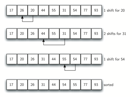
The way in which the increments are chosen is the unique feature of the Shell sort.
#include <iostream>
#include "dscpp/sorting.hpp"   // gapInsertionSort + shellSort
using namespace std;

int main() {
    vector<int> aList = {54, 26, 93, 17, 77, 31, 44, 55, 20};
    shellSort(aList);
    printl(aList);
    return 0;
}
After increments of size 4 the list is 20 26 44 17 54 31 93 55 77
After increments of size 2 the list is 20 17 44 26 54 31 77 55 93
After increments of size 1 the list is 17 20 26 31 44 54 55 77 93
17 20 26 31 44 54 55 77 93
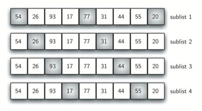
In this case, we begin with $\frac{n}{2}$ sublists. On the next pass, $\frac{n}{4}$ sublists are sorted. Eventually, a single list is sorted with the basic insertion sort.
Although a general analysis of the Shell sort is well beyond the scope of this text, we can say that it tends to fall somewhere between $O(n^2)$ and $O(n)$. By changing the increment, for example using $2^k-1$ (1, 3, 7, 15, 31, and so on), a Shell sort can perform at $O(n^{\frac{3}{2}})$.
7.7 The Merge Sort
We now turn our attention to using a divide and conquer strategy as a way to improve the performance of sorting algorithms. The first algorithm we will study is the merge sort.
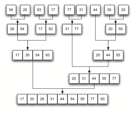
Merge sort is a recursive algorithm that continually splits a list in half. If the list is empty or has one item, it is sorted by definition (the base case). If the list has more than one item, we split the list and recursively invoke a merge sort on both halves.
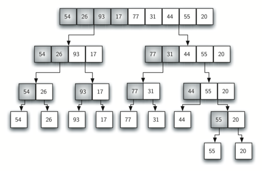
Once the two halves are sorted, the fundamental operation, called a merge, is performed
Merging is the process of taking two smaller sorted lists and combining them together into a single sorted new list.
#include <iostream>
#include "dscpp/sorting.hpp"
using namespace std;

int main() {
    vector<int> aList = {54, 26, 93, 17};
    mergeSort(aList);   // the final Merging line is the sorted result
    return 0;
}
Splitting 54 26 93 17
Splitting 54 26
Splitting 54
Merging 54
Splitting 26
Merging 26
Merging 26 54
Splitting 93 17
Splitting 93
Merging 93
Splitting 17
Merging 17
Merging 17 93
Merging 17 26 54 93
The Splitting/Merging log shows the recursion dividing the vector down to single elements, then merging sorted halves back together.
Once the merge_sort() function is invoked on the left half and the right half (lines 6–7), it is assumed they are sorted. The rest of the function is responsible for merging the two smaller sorted lists into a larger sorted list.
Notice that the merge operation places the items back into the original list (a_list) one at a time by repeatedly taking the smallest item from the sorted lists. The condition in line 13 (left_half[i] <= right_half[j]) ensures that the algorithm is stable. A stable algorithm maintains the order of duplicate items in a list and is preferred in most cases.
In order to analyze the merge_sort() function, we need to consider the two distinct processes that make up its mplementation. First, the list is split into halves. We already computed (in a binary search) that we can divide a list in half $\log n$ times.
The second process is the merge. Each item in the list will eventually be processed and placed on the sorted list. So the merge operation requires $n$ operations in each level.
The result of this analysis is that $\log n$ splits, each of which costs $n$ for a total of $n\log n$ operations. A merge sort is an $O(n\log n)$ algorithm.
Recall that the slicing operator is $O(k)$ where $k$ is the size of the slice. We will need to remove the slice operator. Again, this is possible if we simply pass the starting and ending indices along with the list when we make the recursive call. We leave this as an exercise.
It is important to notice that the merge_sort() function requires extra space to hold the two halves as they are extracted with the slicing operations. This additional space can be a critical factor if the list is large and can make this sort problematic when working on large data sets!
display_quiz(path+"merge.json", max_width=800)
7.8. The Quicksort
The quicksort uses divide and conquer to gain the same advantages as the merge sort, while not using additional storage. As a trade-off, however, it is possible that the list may not be divided in half. When this happens, we will see that performance is diminished.
A quicksort first selects a pivot value. Although there are many different ways to choose the pivot value, we will simply use the first item in the list.
The role of the pivot value is to assist with splitting the list. The actual position where the pivot value belongs in the final sorted list, commonly called the split point, will be used to divide the list for subsequent calls to the quicksort.
In below, 54 will serve as our first pivot value

The partition process will happen next. It will find the split point and at the same time move other items to the appropriate side of the list, either less than or greater than the pivot value.
Partitioning begins by locating two position markers — let's call them left_mark and right_mark — at the beginning and end of the remaining items in the list. The goal of the partition process is to move items that are on the wrong side with respect to the pivot value while also converging on the split point.
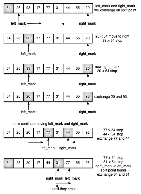
We begin by incrementing left_mark until we locate a value that is greater than the pivot value. We then decrement right_mark until we find a value that is less than the pivot value. At this point we have discovered two items that are out of place with respect to the eventual split point. Now we can exchange these two items and then repeat the process again.
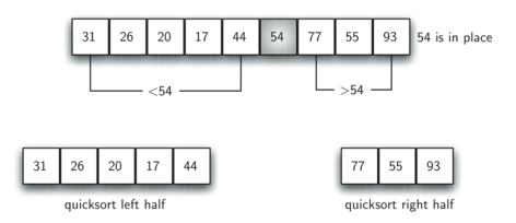
At the point where right_mark becomes less than left_mark, we stop. The position of right_mark is now the split point! The pivot value can be exchanged with the contents of the split point and the pivot value is now in place.
In addition, all the items to the left of the split point are less than the pivot value, and all the items to the right of the split point are greater than the pivot value. The list can now be divided at the split point and the quicksort can be invoked recursively on the two halves!
void quickSort(vector<int>& aList) {
    quickSortHelper(aList, 0, aList.size() - 1);
}

void quickSortHelper(vector<int>& aList, int first, int last) {
    if (first < last) {
        int split = partition(aList, first, last);
        printl(aList);
        quickSortHelper(aList, first, split - 1);
        quickSortHelper(aList, split + 1, last);
    }
}
#include <iostream>
#include "dscpp/sorting.hpp"   // partition + quickSort (md listing above)
using namespace std;

int main() {
    vector<int> aList = {54, 26, 93, 17, 77, 31, 44, 55, 20};
    quickSort(aList);   // prints the vector after every partition
    printl(aList);
    return 0;
}
31 26 20 17 44 54 77 55 93
17 26 20 31 44 54 77 55 93
17 26 20 31 44 54 77 55 93
17 20 26 31 44 54 77 55 93
17 20 26 31 44 54 55 77 93
17 20 26 31 44 54 55 77 93
In order to find the split point, each of the $n$ items needs to be checked against the pivot value. The result is $O(n \log n)$. In addition, there is no need for additional memory as in the merge sort process!
Unfortunately, in the worst case, the split points may not be in the middle and can be very skewed to the left or the right, leaving a very uneven division. In this case, it divides into sorting a list of 0 items and a list of $n-1$ items. Then sorting a list of $n-1$ divides into a list of size 0 and a list of size $n-2$, and so on. The result is an $O(n^2)$ sort with all of the overhead that recursion requires.
We mentioned earlier that there are different ways to choose the pivot value. In particular, we can attempt to alleviate some of the potential for an uneven division by using a technique called median of three.
To choose the pivot value, we will consider the first, the middle, and the last element in the list. In our example, those are 54, 77, and 20. Now pick the median value, in our case 54, and use it for the pivot value.
The idea is that in the case where the first item in the list does not belong toward the middle of the list, the median of three will choose a better "middle" value. This will be particularly useful when the original list is somewhat sorted to begin with. We leave the implementation of this pivot value selection as an exercise.